CATEGORY / MIT Data Science: Data To Insights

03Nov

2016

Eugene / Learning, MIT Data Science: Data To Insights / 0 comment

P-Value

p-value: probability of observing an outcome which is at least as hostile (or adversarial) to the null hypothesis as the one observed

Example
Null hypothesis: mean lifetime of a manufacturing device = 9.4 years
Accepted: within 0.396 units

50 elements with sample mean of 8.96
What is the probability that when we generate a different and independent sample average of 50 observations, we get the value <8.96 if the null hypothesis is true?

Worse than 8.96
1. Getting a number smaller than 8.96
2. Getting a number larger than 9.84

$P(Z\leq-\frac{0.44}{1.43/\sqrt{50}})+P(Z\geq\frac{0.44}{1.43/\sqrt{50}})=2\times P(Z\leq-2.175)=3\%$

Conclusion: the larger the p-value, the stronger the evidence supporting the hypothesis.

03Nov

2016

Eugene / Learning, MIT Data Science: Data To Insights / 0 comment

Validity Of Binomial Distribution

Binomial distribution: discrete probability distribution of the number of successes in a sequence of $n$ independent yes/no experiments, each of which yields success with probability $p$

Null hypothesis: there is no there is no significant difference between specified populations, any observed difference being due to sampling or experimental error

$P(X = k) = \binom n k p^k(1-p)^{n-k}$

$P(X \le k) = \sum_{i=0}^{\lfloor k \rfloor} {n\choose i}p^i(1-p)^{n-i}$

03Nov

2016

Eugene / Learning, MIT Data Science: Data To Insights / 0 comment

Hypothesis Testing

Hypothesis testing: using a data observed from a distribution with unknown parameters, we hypothesise that the parameters of this distribution take particular values and test the validity of this hypothesis using statistical methods

Confidence intervals: provide probabilistic level of certainty regarding parameters of a distribution

Example:
1. $X_1, X_2,..., X_n$
2. unknown mean value $\mu$
3. known $\sigma$

normal distribution: $N(\mu, \sigma^2)$
estimate of $\mu$ : $\bar X=\frac{X_1, X_2,..., X_n}{n}$
distribution of $\bar x$ : $N(\mu, \frac{\sigma^2}{n})$

Suppose:
$P(\bar X\leq \mu+2)$
$P(\bar X-\mu\leq 2)$
$P(\frac{\bar X-\mu}{\sigma/\sqrt{n}}\leq \frac{2}{\sigma/\sqrt{n}})$

03Nov

2016

Eugene / Learning, MIT Data Science: Data To Insights / 0 comment

Types Of Errors

$\begin{array}{|l|l|l|l|} \hline & & \textbf{Predicted fraud?} & \\ \hline & & \textbf{Y} & \textbf{N} \\ \hline {\textbf{Is it actually fraud?}} & \textbf{Y} & +/+ \text{(true positive)} & -/+ \text{(false negative - type 2)} \\ \hline {\textbf{}} & \textbf{N} & +/- \text{(false positive - type 1)} & -/- \text{(true negative)} \\ \hline \end{array}$

Precision: how often a classifier is right when it says something is fraud $(\frac{\text{true positives}}{\text{true positives}+\text{false positives}})$
Recall: how much of the actual fraud that we correctly detect $(\frac{\text{true positives}}{\text{true positives}+\text{false negatives}})$

$\begin{array}{|l|l|} \hline \textbf{Conservation (flag fewer transactions)} & \textbf{Aggressive (flag more transactions)}\\\hline \text{high precision (few false positives)} & \text{low precision (many false positives)}\\\hline \text{low recall (miss some fraud)} & \text{high recall (catch most fraud)}\\\hline \end{array}$

Harmonic mean of $x$ and $y$ $=$ $\frac{1}{\frac{1}{2}(\frac{1}{x}+\frac{1}{y})}$

$F_1$ $=$ $\frac{1}{\frac{1}{2}(\frac{1}{\text{precision}}+\frac{1}{\text{recall}})}=\frac{2\times\text{precision}\times\text{recall}}{\text{precision}+\text{recall}}$

01Nov

2016

Eugene / Learning, MIT Data Science: Data To Insights / 0 comment

Regression Analysis

Definition: discovering correlations between the outcome $y$ and the set of regressors $x$ (features)

$y$ : real random variable
$x$ : vector or random variables $X=(X_1,...,X_p)'$

Example
For wages, suppose
$y$ : hourly wage
$x$ : regressors (experience, gender, education)

$X=(D,W')'$
$D$ : target regressor
$W$ : controls of components

Prediction: how can we use $X$ to predict $Y$ well?
Inference: how does the predicted value of $Y$ change if we change a component of $X$ holding the rest of the components of $X$ fixed?

29Oct

2016

Eugene / Learning, MIT Data Science: Data To Insights / 0 comment

Modularity Clustering

Method: define modularity score that we aim to maximise

Characteristic idea: compare communities to a random baseline graph that shares some properties with the actual graph, such as the number of edges and the degree of the nodes

1. Compute the number of edges within a community, then subtract the expected number of edges as per the baseline model ( $A_{ij}-P_{ij}$ )
2. $A_{ij}=1$ : if edge is between $i,j$
$A_{ij}=1$ : if there is no edge
$P_{ij}=0.26$

Modularity score: $\text{edges in community 1}-\text{baseline expected edges in community 1}+\text{edges in community 2}-\text{baseline expected edges in community 2}$
If score is large, then community is dense

Process:
1. Start with some partitioning, then move nodes between the groups to see if it improves the score
2. Use eigenvectors

29Oct

2016

Eugene / Learning, MIT Data Science: Data To Insights / 0 comment

Spectral Clustering

1. Create neighbourhood graph
2. Compute laplacian
3. Compute eigenvectors of laplacian, the ones with the smallest eigenvalues give new features
4. Run k-means clustering on new features

29Oct

2016

Eugene / Learning, MIT Data Science: Data To Insights / 0 comment

Eigenvectors

To capture global connectivity structure, eigenvectors are really useful. Results will be spectral clustering.

Spectrum of matrix: set of eigenvalues
Matrix: Laplacian of graph

Labelled graph:

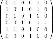
Adjacency matrix: $\left(\begin{array}{rrrrrr} 0 & 1 & 0 & 0 & 1 & 0\\ 1 & 0 & 1 & 0 & 1 & 0\\ 0 & 1 & 0 & 1 & 0 & 0\\ 0 & 0 & 1 & 0 & 1 & 1\\ 1 & 1 & 0 & 1 & 0 & 0\\ 0 & 0 & 0 & 1 & 0 & 0\\ \end{array}\right)$

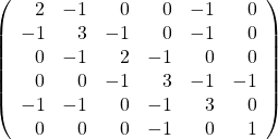
Laplacian matrix: $\left(\begin{array}{rrrrrr} 2 & -1 & 0 & 0 & -1 & 0\\ -1 & 3 & -1 & 0 & -1 & 0\\ 0 & -1 & 2 & -1 & 0 & 0\\ 0 & 0 & -1 & 3 & -1 & -1\\ -1 & -1 & 0 & -1 & 3 & 0\\ 0 & 0 & 0 & -1 & 0 & 1\\ \end{array}\right)$

22Oct

2016

Eugene / Learning, MIT Data Science: Data To Insights / 0 comment

Clusters

Cluster: points that are well-connected with each other (lots of edges)
Number of edges = volume
Volume per node = density
Cut value: separation of clusters
Cut(C) = 1 (number of edges between clusters)

1^st criteria: density must be large
2^nd criteria: there should not be too many edges between different clusters

Normalised Cut
$\text{Ncut(C)}=\frac{\text{Cut(C)}}{\text{Volume(C)}\times \text{Volume(V\C)}}$

Conductance
$\text{conductance(C)}=\frac{\text{Cut(C)}}{\text{Min\{Volume(C),Volume(V\C)\}}}$

Good clusters are not too small, internally well-connected and separated from the rest of the nodes

22Oct

2016

Eugene / Learning, MIT Data Science: Data To Insights / 0 comment

Principal Component Analysis

Patterns = principal component = vector
Finds major axis of variation in data
Each data point expressed as a linear combination of patterns

$Ax=\lambda x$
$\text{Matrix}\times\text{eigenvector}=\text{eigenvalue}\times\text{eigenvector}$
Eigenvectors capture major direction that are inherent in the matrix
The larger the eigenvalue, the more important is the vector
Covariance matrix contains terms for all positive pairs of features

- PAGE 1 OF 2 -