CATEGORY / Stanford Machine Learning

01Dec

2016

Eugene / Learning, Stanford Machine Learning / 0 comment

Control Statements (Octave)

1. for i=1:10,
v(i) = 2^i;
end;
v
$v=\begin{pmatrix} 2\\ 4\\ 8\\ 16\\ 32\\ 64\\ 128\\ 256\\ 512\\ 1024 \end{pmatrix}$

2. i=1;
while i<=5,
v(i) = 100;
i = i+1;
end;
v
$v=\begin{pmatrix} 100\\ 100\\ 100\\ 100\\ 100\\ 64\\ 128\\ 256\\ 512\\ 1024 \end{pmatrix}$

3. i=1;
while true,
v(i) = 999;
i = i+1;
if i==7;;
break;
end;
end;
v
$v=\begin{pmatrix} 999\\ 999\\ 999\\ 999\\ 999\\ 999\\ 128\\ 256\\ 512\\ 1024 \end{pmatrix}$

4. v(1) = 2;
if v(1) == 1,
disp('The value is one');
elseif v(1) == 2,
disp('The value is two');
else
disp('The value is not one or two');
end;
The value is two

26Nov

2016

Eugene / Learning, Stanford Machine Learning / 0 comment

Plotting Data (Octave)

1. t=[0:0.01:0.98]
$t=\begin{pmatrix} 0 & 0.01 & 0.02 & ... & 0.98 \end{pmatrix}$

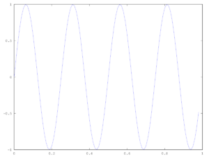
2. y1 = sin(2*pi*4*t)
plot(t,y1)
sine

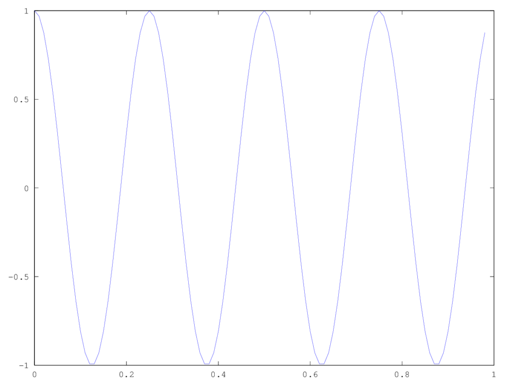
3. y2 = cos(2*pi*4*t)

plot(t,y2)
cosine

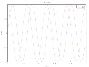
4. plot(t,y1);
hold on;
plot(t,y2,'r');
xlabel('time')
ylabel('value')
legend('sin','cos')
title('my plot')
myplot

26Nov

2016

Eugene / Learning, Stanford Machine Learning / 0 comment

1. A = [1 2; 3 4; 5 6]
$A=\begin{pmatrix} 1 & 2 \\ 3 & 4 \\ 5 & 6 \end{pmatrix}$
B = [11 12; 13 14; 15 16]
$B=\begin{pmatrix} 11 & 12 \\ 13 & 14 \\ 15 & 16 \end{pmatrix}$
C = [1 1; 2 2]
$C=\begin{pmatrix} 1 & 1 \\ 1 & 2 \end{pmatrix}$

2. A*C
$\begin{pmatrix} 5 & 5\\ 11 & 11 \\ 17 & 17 \end{pmatrix}$

3. A .* B take each element of A to multiply by each element of B
$\begin{pmatrix} 11 & 24\\ 39 & 56 \\ 75 & 96 \end{pmatrix}$

4. A .^ 2 square each element of A
$\begin{pmatrix} 1 & 4\\ 9 & 16 \\ 25 & 36 \end{pmatrix}$

5. v = [1; 2; 3]
$v=\begin{pmatrix} 1\\ 2\\ 3 \end{pmatrix}$

6. 1 ./ v element-wise reciprocal of v
$v=\begin{pmatrix} 1.00000\\ 0.50000\\ 0.33333 \end{pmatrix}$

7. log(v) element-wise logarithm of v
exp(v) element-wise exponential of v
abs(v) element-wise absolute value of v
-v element-wise negative value of v
v+1 element-wise addition of 1 to v

8. A = [1 2; 3 4; 5 6]
$A=\begin{pmatrix} 1 & 2 \\ 3 & 4 \\ 5 & 6 \end{pmatrix}$
A' transpose of A
$\begin{pmatrix} 1 & 2 & 3 \\ 4 & 5 & 6 \end{pmatrix}$

9. w = [1 15 2 0.5]
$w=\begin{pmatrix} 1 & 15 & 2 & 0.5 \end{pmatrix}$

10. max (w) maximum value of w
val = 15

11. [val, ind] = max(w) maximum value of w and index where it is located
val = 15
ind = 2

12. w < 3 element-wise comparison of whether w is less than 3
$\begin{pmatrix} 1 & 0 & 1 & 1 \end{pmatrix}$

13. find(w < 3) find which elements that variable w is less than 3
$\begin{pmatrix} 1 & 3 & 4 \end{pmatrix}$

14. sum(w) sum of w
ans = 18.5

15. prod(w) product of w
ans = 15

16. floor(w) rounds down elements of w
$\begin{pmatrix} 1 & 15 & 2 & 0 \end{pmatrix}$

17. ceil(w) rounds down elements of w
$\begin{pmatrix} 1 & 15 & 2 & 1 \end{pmatrix}$

18. A = magic(3) magic square of 3 by 3
$\begin{pmatrix} 8 & 1 & 6\\ 3 & 5 & 7\\ 4 & 9 & 2 \end{pmatrix}$

19. [r,c] = find(A >= 7) find rows and columns of A greater than or equal to 7
$r=\begin{pmatrix} 1\\ 3\\ 2 \end{pmatrix}$
$c=\begin{pmatrix} 1\\ 2\\ 3 \end{pmatrix}$

20. A(2,3)
$\begin{pmatrix} 7 \end{pmatrix}$

21. max(A,[],1) column-wise maximum of A
$\begin{pmatrix} 8 & 9 & 7 \end{pmatrix}$

22. max(A,[],2) row-wise maximum of A
$\begin{pmatrix} 8 \\ 7 \\ 9 \end{pmatrix}$

23. max(max(A))
$\begin{pmatrix} 9 \end{pmatrix}$

24. pinv(A) inverse of A
$\begin{pmatrix} 0.147 & -0.144 & 0.064 \\ -0.061 & 0.022 & 0.106 \\ -0.019 & 0.189 & -0.103 \end{pmatrix}$

16Nov

2016

Eugene / Learning, Stanford Machine Learning / 0 comment

Moving Data (Octave)

Matrices
1. A = [1 2; 3 4; 5 6]
$A=\begin{pmatrix} 1 & 2 \\ 3 & 4 \\ 5 & 6 \end{pmatrix}$

2. size(A) size of matrix
$\begin{matrix} 3 & 2 \end{matrix}$

3. size(A,1) number of rows
ans = 3

4. size(A,2) number of columns
ans = 2

5. A(3,2) $A_{32}$
ans = 6

6. A(2,:) every element along row 2
$\begin{pmatrix} 3 & 4 \end{pmatrix}$

7. A(:,1) every element along column 1
$\begin{pmatrix} 1\\ 3\\ 5 \end{pmatrix}$

8. A([1 3],:) every element along rows 1 and 3
$\begin{pmatrix} 1 & 2\\ 5 & 6 \end{pmatrix}$

9. A(:,2) = [10; 11; 12] replace column 2 with new elements
$\begin{pmatrix} 1 & 10 \\ 3 & 11 \\ 5 & 12 \end{pmatrix}$

10. A = [A, [100; 101; 102]] append new column vector to the right
$\begin{pmatrix} 1 & 10 & 100 \\ 3 & 11 & 101\\ 5 & 12 & 102 \end{pmatrix}$

11. A(:) put all elements of A into a single vector
$\begin{pmatrix} 1\\ 3\\ 5\\ 10\\ 11\\ 12\\ 100\\ 101\\ 102 \end{pmatrix}$

12. A = [1 2; 3 4; 5 6]
B = [11 12; 13 14; 15 16]
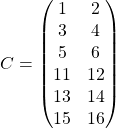
C = [A B] concatenating A and B
$C=\begin{pmatrix} 1 & 2 & 11 & 12 \\ 3 & 4 & 13 & 14\\ 5 & 6 & 15 & 16 \end{pmatrix}$

13. C = [A; B] putting A on top of B
$C=\begin{pmatrix} 1 & 2 \\ 3 & 4 \\ 5 & 6 \\ 11 & 12 \\ 13 & 14 \\ 15 & 16 \end{pmatrix}$

14. v = [1 2 3 4]
$v=\begin{pmatrix} 1 & 2 & 3 & 4 \end{pmatrix}$

15. length(v) length of vector v
ans = 4

Loading files
1. path: pwd shows where Octave location is

2. change directory: cd '/Users/eugene/desktop'

3. list files: ls

4. load files: load featuresfile.dat

5. list particular file: featuresfile

6. check saved variables: who

7. check saved variables (detailed view): whos

8. clear particular variable: clear featuresfile

9. clear all: clear

10. restrict particular variable: v = featuresfile(1:10) only first 10 elements from featuresfile

11. save variable into file: save testfile.mat v variable v is saved into testfile.mat

12. save variable into file: save testfile.txt v -ascii variable v is saved into text file

16Nov

2016

Eugene / Learning, Stanford Machine Learning / 0 comment

Basic Operations (Octave)

Logical operations
1. 1 == 2 1 equals to 2
ans = 0 false

2. 1 ~= 2 1 is not equal to 2
ans = 0 true

3. 1 && 2 AND
ans = 0

4. 1 || 2 OR
ans = 1

5. xor(1,0)
ans = 1

Change default octave prompt: PS1('>> ');

Assign variables
1. a = 3 printing out a = 3

2. a = 3; suppress print out

3. b = 'hi' for strings

4. c = (3>=1) true

Printing
1. disp(a) to show a

2. a = pi
disp(sprintf('2 decimals: %0.2f', a)) 2 decimal places
2 decimals: 3.14

2. disp(sprintf('2 decimals: %0.6f', a)) 6 decimal places
2 decimals: 3.141593

3. format long
a
a = 3.14159265358979

4. format short
a
a = 3.1416

Matrices
1. A = [1 2; 3 4; 5 6] 3 by 2 matrix
$A=\begin{pmatrix} 1 & 2 \\ 3 & 4 \\ 5 & 6 \end{pmatrix}$

2. v = [1 2 3] 1 by 3 matrix (row vector)
$v=\begin{pmatrix} 1 & 2 & 3 \end{pmatrix}$

3. v = [1; 2; 3] 3 by 1 matrix (column vector)
$v=\begin{pmatrix} 1\\ 2\\ 3 \end{pmatrix}$

4. v=1:0.1:2 1 by 11 matrix (row vector)
$v=\begin{pmatrix} 1 & 1.1 & 1.2 & ... & 1.9 & 2 \end{pmatrix}$

5. v=1:6 1 by 6 matrix (row vector)
$v=\begin{pmatrix} 1 & 2 & 3 & 4 & 5 & 6 \end{pmatrix}$

6. ones(2,3) 2 by 3 matrix of ones
$\begin{pmatrix} 1 & 1 & 1\\ 1 & 1 & 1 \end{pmatrix}$

7. 2*ones(2,3)
$\begin{pmatrix} 2 & 2 & 2\\ 2 & 2 & 2 \end{pmatrix}$

8. zeros(2,3) 2 by 3 matrix of zeroes
$\begin{pmatrix} 0 & 0 & 0\\ 0 & 0 & 0 \end{pmatrix}$

9. rand(2,3) 2 by 3 matrix of random numbers between 0 and 1

10. randn(2,3) 2 by 3 matrix of random numbers drawn from a Gaussian distribution with mean 0 and variance

11. eye(4) 4 by 4 identity matrix
$\begin{pmatrix} 1 & 0 & 0 & 0\\ 0 & 1 & 0 & 0\\ 0 & 0 & 1 & 0\\ 0 & 0 & 0 & 1 \end{pmatrix}$

Plot histogram: w = -6 + sqrt(10)*(randn(1,10000))
hist(w) histogram
hist(w,50) histogram with 50 bins

Help: help rand help function

15Nov

2016

Eugene / Learning, Stanford Machine Learning / 0 comment

Normal Equation

$\theta = (X^T X)^{-1}X^T y$

Advantages and disadvantages:
1. No need to choose $\alpha$
2. Don’t need to iterate
3. Need to compute $(X^TX)^{-1}$
4. Slow if $n$ is very large

If $X^TX$ is non-invertible:
1. Redundant features (linearly dependent)
2. Too many features (e.g. $m\le n$ )
a. delete some features
b. use regularisation

14Nov

2016

Eugene / Learning, Stanford Machine Learning / 0 comment

Application Of Gradient Descent

Feature scaling: get every feature into approximately a $-1 \le x_i \le 1$ range

Mean normalisation: replace $x_i$ with $x_i-\mu_i$ to make features have approximately zero mean (do not apply to $x_0=1$ )

$x_i := \dfrac{x_i - \mu_i}{s_i}$
$\mu_i$ : average value of $x_i$ in the training set
$s_1$ : standard deviation

Points to note:
1. If gradient descent is working correctly, $J(\theta)$ should decrease after each iteration.
2. If $\alpha$ is too small, we will have slow convergence.
3. If $\alpha$ is too large, $J(\theta)$ may not converge.

Advantages and disadvantages:
1. Need to choose $\alpha$
2. Needs many iterations
3. Works well even when $n$ is large

14Nov

2016

Eugene / Learning, Stanford Machine Learning / 0 comment

Gradient Descent For Multiple Variables

Cost function: $J(\theta) = \dfrac {1}{2m} \displaystyle \sum_{i=1}^m \left (h_\theta (x^{(i)}) - y^{(i)} \right)^2$
$J(\theta) = \dfrac {1}{2m} \displaystyle \sum_{i=1}^m \left (\theta^Tx^{(i)} - y^{(i)} \right)^2$
$J(\theta) = \dfrac {1}{2m} \displaystyle \sum_{i=1}^m \left ( \left( \sum_{j=0}^n \theta_j x_j^{(i)} \right) - y^{(i)} \right)^2$

Gradient descent:

$ <img src="https://teach.sg/wp-content/ql-cache/quicklatex.com-180d38ebaaff2b28806bdd8feee8e5ee_l3.png" height="50" width="632" class="ql-img-displayed-equation quicklatex-auto-format" alt="\begin{align*} & \text{repeat until convergence:} \; \lbrace \newline \; & \theta_j := \theta_j - \alpha \frac{1}{m} \sum\limits_{i=1}^{m} (h_\theta(x^{(i)}) - y^{(i)}) \cdot x_j^{(i)} \; & \text{for j := 0..n} \newline \rbrace \end{align*}" title="Rendered by QuickLaTeX.com"/>$

which breaks down into

$ <img src="https://teach.sg/wp-content/ql-cache/quicklatex.com-ade19e57866347ec87a2a0df45d0c145_l3.png" height="50" width="1189" class="ql-img-displayed-equation quicklatex-auto-format" alt="\begin{align*} & \text{repeat until convergence:} \; \lbrace \newline \; & \theta_0 := \theta_0 - \alpha \frac{1}{m} \sum\limits_{i=1}^{m} (h_\theta(x^{(i)}) - y^{(i)}) \cdot x_0^{(i)}\newline \; & \theta_1 := \theta_1 - \alpha \frac{1}{m} \sum\limits_{i=1}^{m} (h_\theta(x^{(i)}) - y^{(i)}) \cdot x_1^{(i)} \newline \; & \theta_2 := \theta_2 - \alpha \frac{1}{m} \sum\limits_{i=1}^{m} (h_\theta(x^{(i)}) - y^{(i)}) \cdot x_2^{(i)} \newline & \cdots \newline \rbrace \end{align*}" title="Rendered by QuickLaTeX.com"/>$

14Nov

2016

Eugene / Learning, Stanford Machine Learning / 0 comment

Linear Regression With Multiple Variables

Notation:
$n$ : number of features
$x^{(i)}$ : input (features) of $i^{th}$ training example
$x^{(i)}_j$ : value of feature $j$ in $i^{th}$ training example

$h_\theta (x) = \theta_0 + \theta_1 x_1 + \theta_2 x_2 + \theta_3 x_3 + \cdots + \theta_n x_n$

$ <img src="https://teach.sg/wp-content/ql-cache/quicklatex.com-06f129ca3a97efd2c74e813c392da568_l3.png" height="32" width="384" class="ql-img-displayed-equation quicklatex-auto-format" alt="\begin{align*} h_\theta(x) = \begin{bmatrix} \theta_0 \hspace{2em} \theta_1 \hspace{2em} ... \hspace{2em} \theta_n \end{bmatrix} \begin{bmatrix} x_0 \newline x_1 \newline \vdots \newline x_n \end{bmatrix} = \theta^T x \end{align*}" title="Rendered by QuickLaTeX.com"/>$

14Nov

2016

Eugene / Learning, Stanford Machine Learning / 0 comment

Matrix Inverse & Transpose

Matrix inverse: If $A$ is an $m\times m$ matrix, and if it has an inverse, then $A\times A^{-1}=A^{-1}\times A=I$
$A=\begin{bmatrix} a & b \newline c & d \newline \end{bmatrix}$
$A^{-1}=\frac{1}{ad-bc}\begin{bmatrix} d & -b \newline -c & a \newline \end{bmatrix}$
Note: Matrices that do not have an inverse are singular or degenerate.

Matrix transpose: Let $A$ be an $m\times n$ matrix, and let $B=A^T$ . then B is an $n\times n$ matrix and $B_{ij}=A_{ji}$ .
$A = \begin{bmatrix} a & b \newline c & d \newline e & f \end{bmatrix}$
$A^T = \begin{bmatrix} a & c & e \newline b & d & f \newline \end{bmatrix}$

- PAGE 1 OF 2 -